Must-Know Google Sheets Formulas for SEO

An Introduction to Google Sheets for SEO
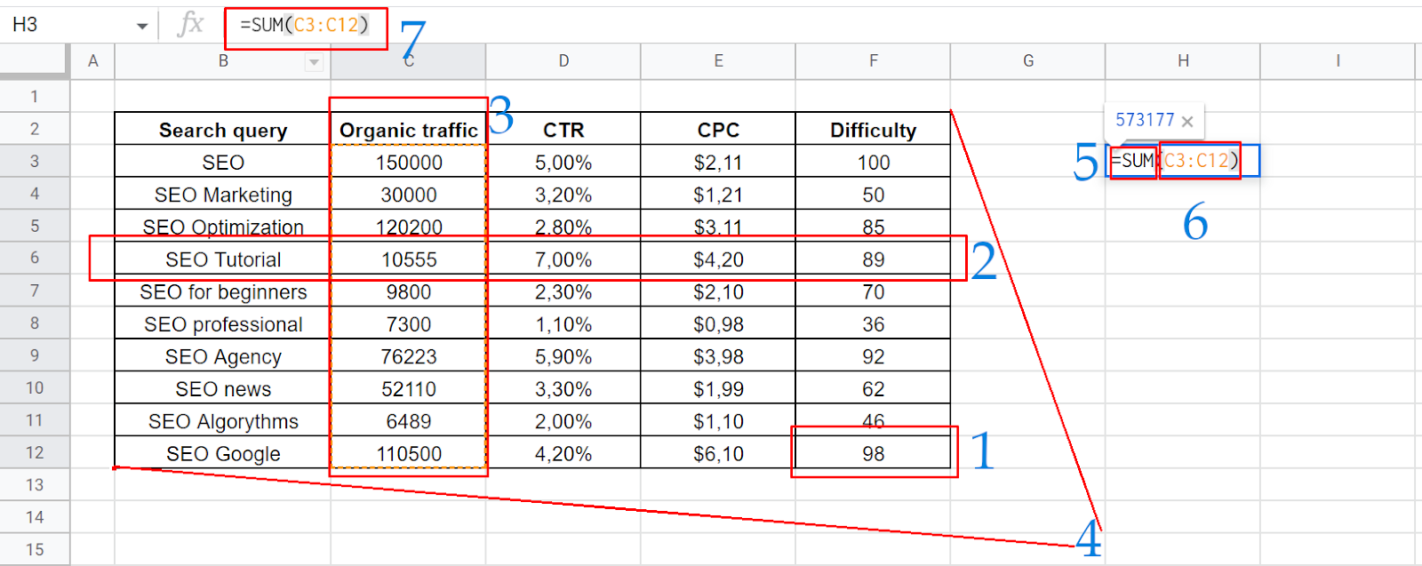
This online app is very similar to Microsoft Excel. It has a similar interface, editing, and formatting tools and also supports formulas and scripts. If you’ve already worked in Excel, you just need to get used to the different syntax. Beginners who will be working with spreadsheets for the first time should familiarize themselves with the basic concepts:
- Cell — a unit of info content, a field where you enter data.
- Line — a horizontal array of cells.
- Column — a vertical array of cells.
- Table — a rectangular array that contains a certain number of columns and rows.
- Function — an operation with data in cells designed to give a specific result.
- Row — a part of the table that the function accesses.
- Formula — a combination of functions and the rows they refer to. In both Microsoft Excel and Google Sheets, formulas begin with the equation sign “=”.
To visualize these concepts, please look at the example below:
Basic SEO Google Sheets Formulas
Basic formulas can significantly increase productivity. If you use them in your daily work, you will decrease your overall workload. As a result, you’ll have more time to conclude your analysis and make important decisions.
IF to See If the Condition Is True or False
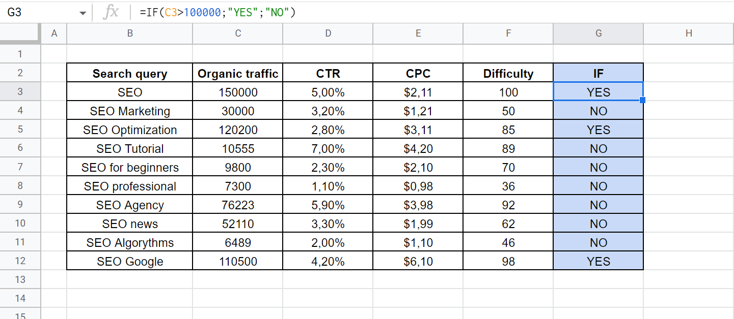
How it works: The formula produces one of two answers depending on whether a certain condition is met in the specified cell.
Syntax: = IF(condition, value_if_true, value_if_false), where:
- condition — a condition expressed as a mathematical function;
- value_if_true — the value if the data in the cell meets the condition;
- value_if_false — value if the condition is not met.
For example, we want to check if the monthly volume of organic traffic exceeds 100 thousand queries. Our SEO formula in Google Sheets will look like this:
=IF(C3>100000;”YES”;”NO”)
You can use various mathematical signs in the condition element:
- equal (=)
- less-than (<)
- greater-than (>)
- less-than-or-equal-to sign (<=)
- greater-than-or-equal-to sign (>=)
- not equal (<>)
Moreover, you should pay attention to the syntax for writing value_if elements. To display text in a cell, be sure to quote it. If you don’t, Google Sheets will treat the value as a formula. In this case, plain text will be recognized as a false function.
LEN to Count the Number of Characters in a Cell
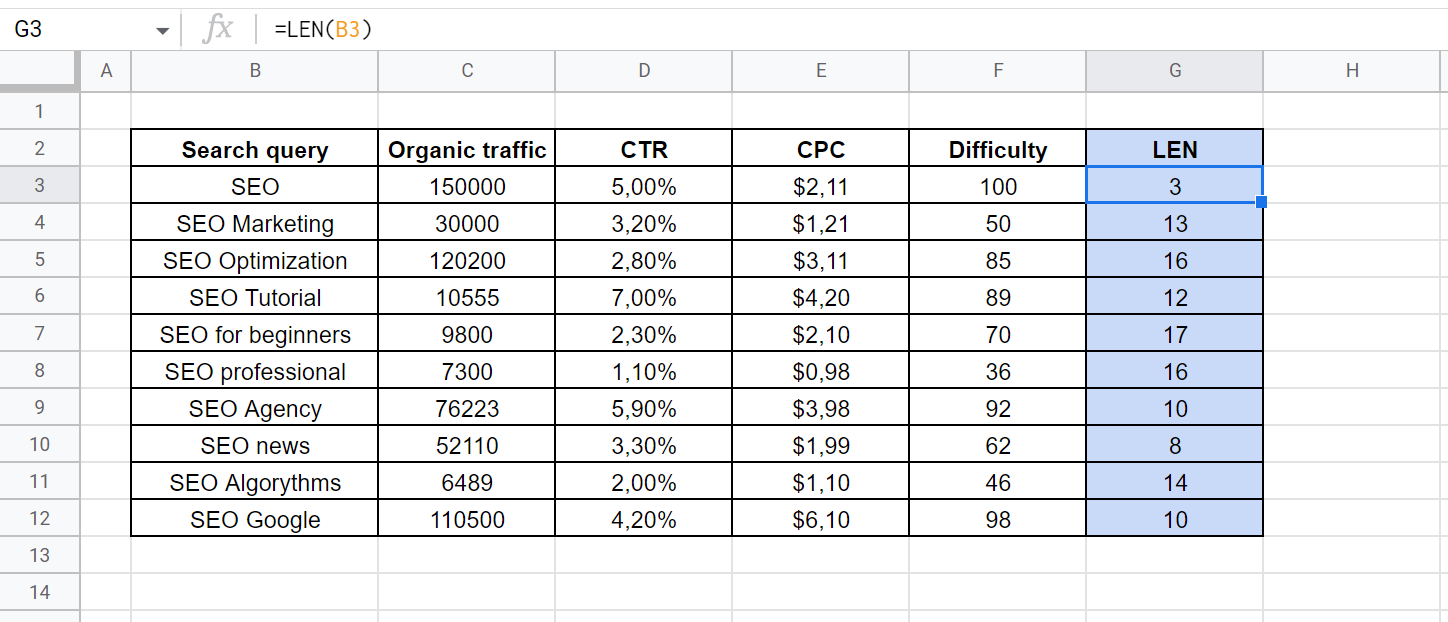
How it works: The formula determines the length of the text in the specified cell. If it contains a formula, the characters it produces as a result are counted.
Syntax: =LEN(insertcell), where:
- insertcell — a cell reference.
For example, we need to count the number of characters in search queries. It is a very valuable SEO metric because it allows you to sort your keywords and check them for compliance with the terms of search engines or contextual advertising platforms. The formula will look like this:
=LEN(B3)
A useful tip: You don’t have to enter a separate formula in each row. After you fill in the first cell, Google Sheets will prompt you to fill in the rest. You just need to agree to use this feature.
SPLIT To Split the Data into Multiple Cells
How it works: The formula splits text and writes it in several cells based on the specified delimiter.
Syntax: =SPLIT(Text, Delimiter), where:
- text — a cell reference that contains the desired text;
- delimiter — a separation character.
For example, we need to highlight certain words from search queries. We can do it by splitting the text into spaces in phrases. The formula will look like this:
=SPLIT(B3; “ ”)
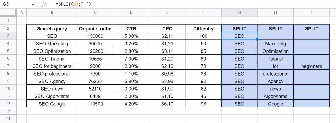
Please note: you should quote the character that is used to separate the text. After executing the function, the formulas will remain only in the leftmost cells of the array. The rest will be written in text. However, if the data changes, it will be updated automatically.
CONCATENATE To Merge Data
How it works: The function generates the content of one cell based on the text in several other cells. Moreover, you can add to it other pieces that aren’t recorded in your table.
Syntax: =CONCATENATE(range1; range2;…), where:
- Range — a reference to cells or data lines. You can add your text instead and quote it.
For example, we want to combine the search query and the volume of organic traffic by separating them with an underscore “_”. The formula will look like this:
=CONCATENATE(B3;“_”;C3)
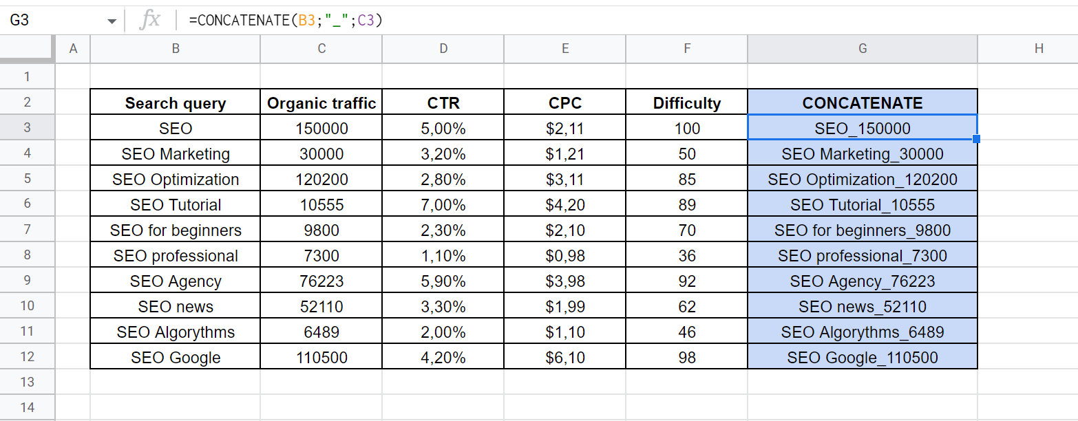
A useful tip: This formula is ideal for merging a page address with a domain name and an HTTP or HTTPS prefix. It simplifies the construction of URLs from fragments uploaded by some SEO services.
COUNTIF for Counting Cells Accordingt Specific Criteria
How it works: Unlike IF, it checks whether a condition is met in a row rather than in a single cell. It shows the number of cells in which the condition is met.
Syntax: =COUNTIF(range, criteria), where:
- range — a reference to data lines;
- criteria — a condition expressed by a mathematical function.
For example, we want to count the number of keywords with a cost per click in contextual advertising up to $2. The formula will look like this:
=COUNTIF(E3:E12; “<2”)
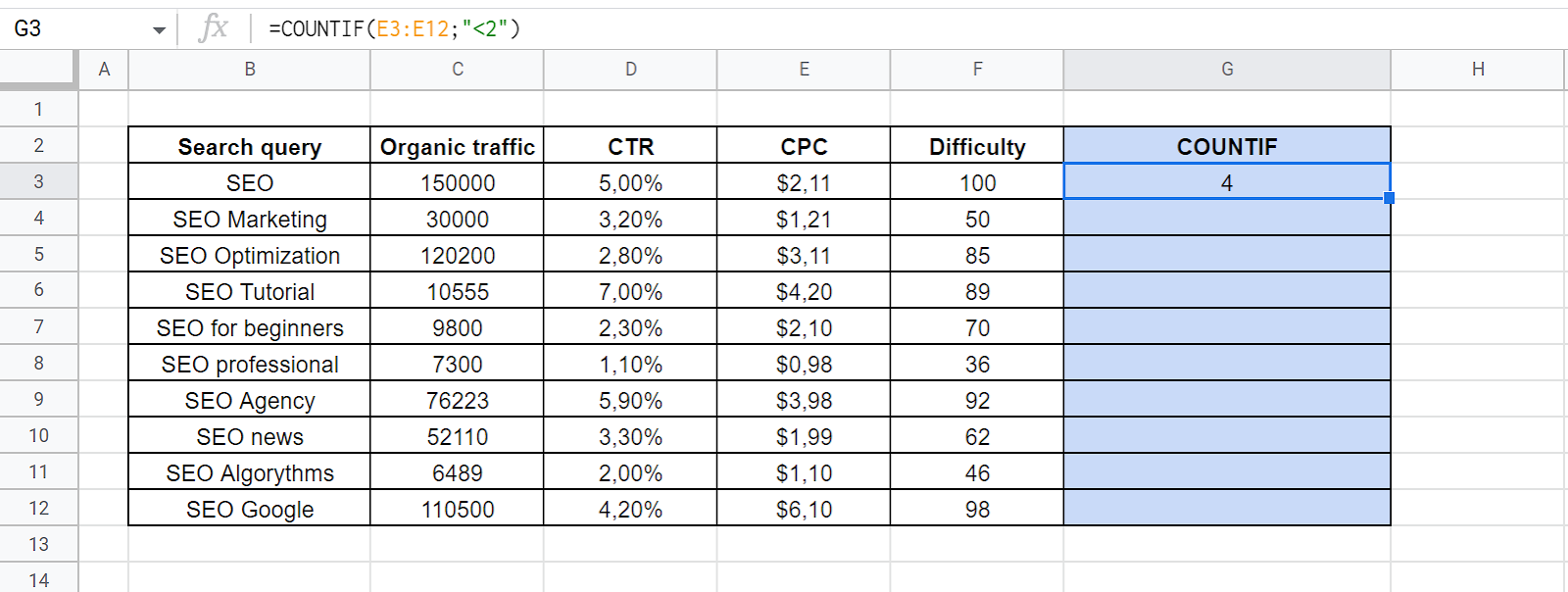
Don’t forget to quote the condition. Moreover, you should keep in mind that you can use equality or inequality operators.
UPPER/LOWER/PROPER to Convert the Text Case
How it works: It changes the case to uppercase, lowercase, or uppercase in the first letter and lowercase in the rest.
Syntax: =UPPER(text), =LOWER(text), =PROPER(text), where:
- Text — a reference to a cell or a manually entered text fragment.
For example, we need to format automatically downloaded suggestions of titles or Description meta tags. Some programs output lowercase letters by default, and some output uppercase letters. In our table, we will first convert the text to lowercase, then to uppercase, and then to the correct spelling. The formulas will look like this:
=LOWER(B3)
=UPPER(G3)
=PROPER(H3)
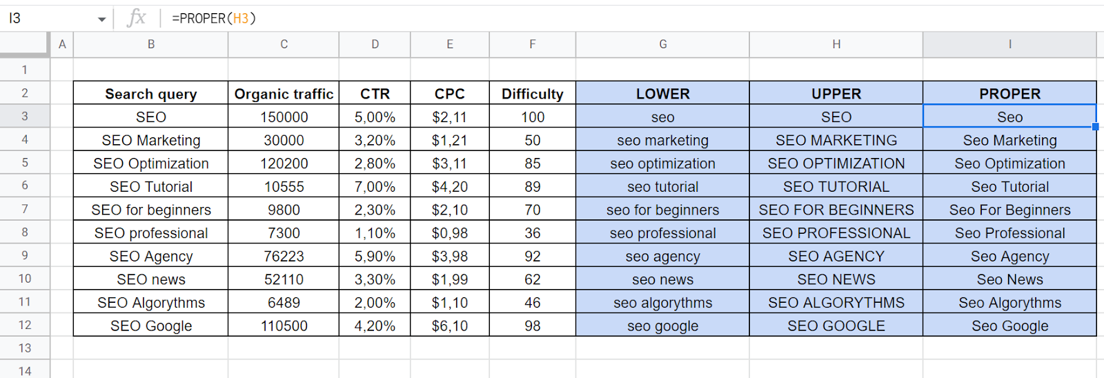
These formulas are also suitable for reporting. Easy formatting allows you to quickly create suitable and well-looking tables that demonstrate your goals or results.
UNIQUE To Find and Remove Duplicates
How it works: It checks a column. If it contains cells with duplicate data, it displays them only once.
Syntax: =UNIQUE(range), where:
- range — the data lines you are viewing.
For example, we have copied the keywords for several pages of our website into one column and want to select all unique values without duplicates. The formula will look like this:
=UNIQUE(B3:B12)
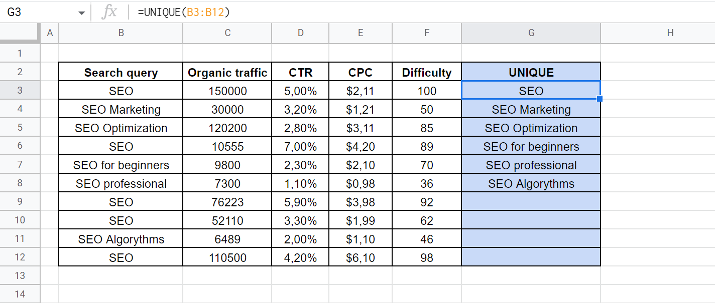
A helpful tip: You can also use the UNIQUE function to delete blank cells. In this case, you can even give a reference to the column. The Google Sheets SEO formula will look like this: =UNIQUE(B:B).
SUMIF to Find Category Totals With
How it works: It checks whether the condition in this cell or another parallel data line is met. If so, it adds it to the total, if not — omits it.
Syntax: =SUMIF(range, criterion, [sum_range]), where:
- range — a row in which the condition is checked;
- criterion — a condition specified by a mathematical function;
- [sum_range] — a row to be added. It is an optional parameter that is entered only if a parallel row is checked for compliance with the condition.
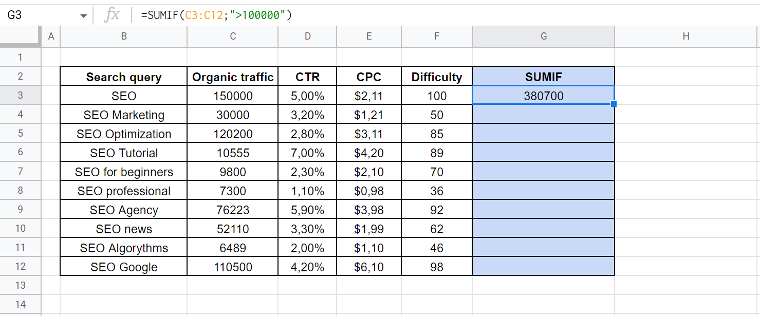
For example, we need to check how much organic traffic is generated by high-frequency keywords that have over 100 thousand views. The formula will look like this:
=SUMIF(C3:C12;”>100000″)
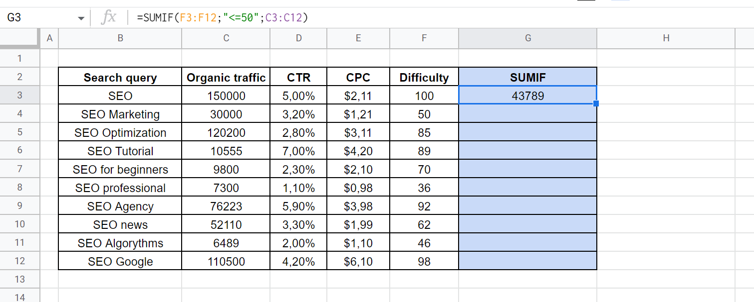
If we want to calculate organic traffic for all queries whose optimization complexity does not exceed 50, we will need a different formula:
=SUMIF(F3:F12;”<=50″;C3:C12)
IFERROR to Set a Default for Error
How it works: If a formula performs an invalid action, this function detects the error and replaces it with another action. It enters text or switches to an alternative formula.
Syntax: =IFERROR(original_formula, value_if_error), where:
- original_formula — the formula you are checking for errors;
- value_if_error — the action to take if an error is found.
For example, the CTR for some keywords is not available owing to the limited functionality of the program or the data lack in the search engine. Instead of a number, these cells are marked with dashes. When we try to calculate, we will get an error notification. To replace it with the “NO DATA” text, you should use the following formula:
=IFERROR(C3*D3; “NO DATA”)
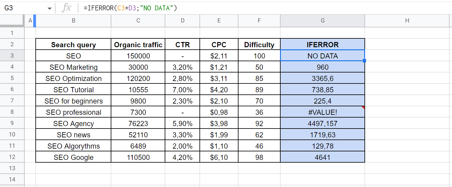
In the screenshot, you can see the error notification in the G8 cell. The IFERROR formula can also work with such errors as #DIV/0! and #ERROR!
TODAY to Add Dates
How it works: It displays the current date in the format set by default in Google Sheets cloud service.
Syntax: =TODAY(). Please note: the function has no parameters and does not refer to cells or rows.
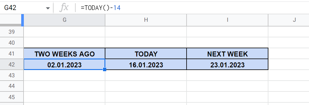
For example, you keep forgetting to update the date in a report. Instead of entering it manually, you can use a simple formula. Using additional mathematical operators, you can subtract a certain number of days from it. For example, we need to know what date was two weeks ago and will be next week on the same day. Simply use the following formulas:
=TODAY()-14
=TODAY()+7
SEARCH for a Specific Value
How it works: It checks if a given text fragment is contained in a certain cell. If so, it numbers the character it starts with.
Syntax: =SEARCH(search_query, text_to_search), where:
- search_query — a text fragment to be found or a cell reference where it is contained;
- text_to_search — a cell reference in which the search is performed.
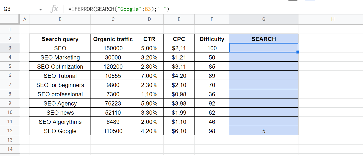
This function can be used to check cells for a specific text. For example, we need to find a key phrase that contains the word “Google.” To get rid of the error notifications, you should use the IFERROR formula discussed above. The final result will look like this:
=IFERROR(SEARCH(“Google”;B3); “ ”)
SORT Your Cells Easily
How it works: It sorts cells in a specific row by the values contained in the same or a parallel row.
Syntax: =SORT(range, sort_column, is_ascending), where:
- range — the row to be sorted;
- sort_column — a row with a characteristic by which the sorting is performed. It can be the same as the previous one;
- is_ascending — the sorting method. If it is performed in ascending order, specify TRUE, in descending order — FALSE.
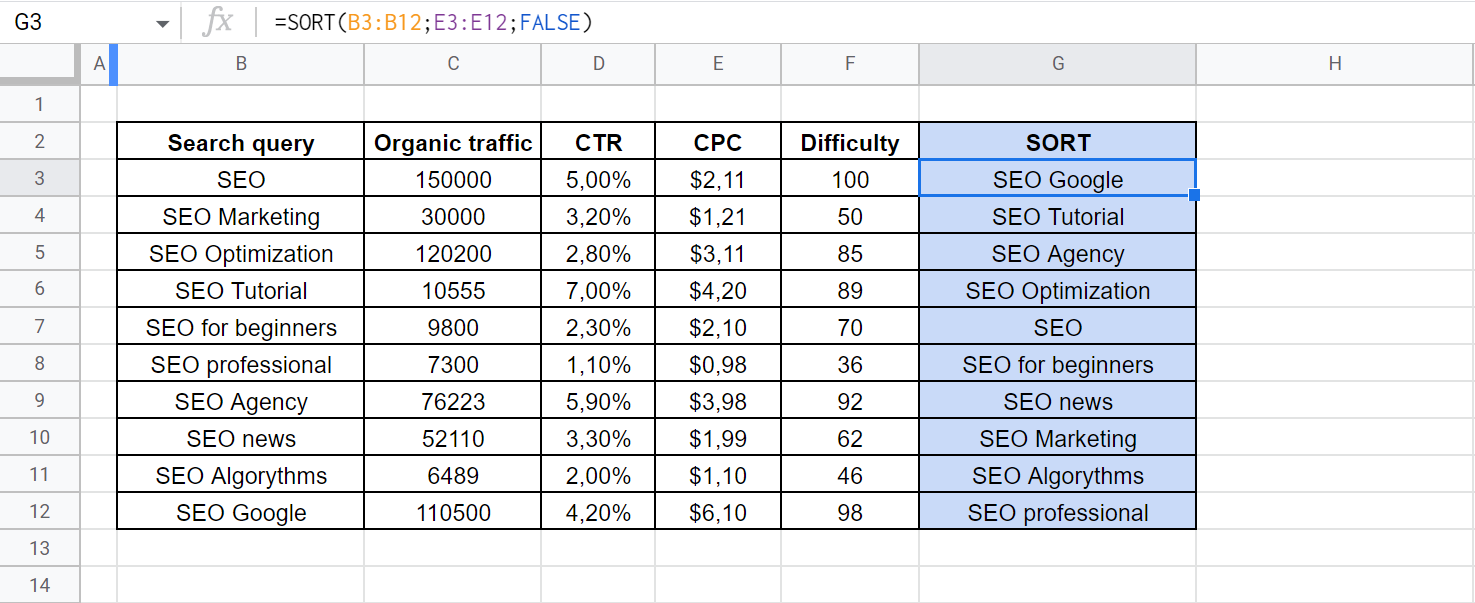
For example, we need to sort keywords by cost per click in contextual advertising. The formula of descending sorting will look like this:
=SORT(B3:B12;E3:E12;FALSE)
Please note: you can enter a formula in one cell only. The column below is filled and updated automatically.
Advanced Google Sheet Formulas For SEOs
A cloud-based spreadsheet service can be a workable alternative to a paid analytics service. You can use it to search for data in large arrays and import info from external sources. However, you will have to master more complex formulas to do it.
IMPORTRANGE for Easy Data Import from Different Files
How it works: It creates a reference between two files. If you change the info in the source, it will be changed in your worksheet.
Syntax: =IMPORTTRANGE(spreadsheet_url, range_string), where:
- spreadsheet_url — a reference to the desired file;
- range_string — addressing of the data series, which contains the name of the page and the array of cells.
For example, we want to import a spreadsheet with keywords, organic traffic volume, and optimization complexity into our file. To create a formula, you will need to find the URL, page name, and array address. It can look like this:
=IMPORTRANGE(“https://docs.google.com/spreadsheets/d/AAAAAAAAAA”, Workplace!A1:C100”).
Please, pay attention to a few nuances:
- You must quote URL and an array address.
- The page name is separated by an exclamation mark.
- If you need to fully import several columns, you should specify only their names without numbers. For example, “Workplace!A:C”.
VLOOKUP to Import Data from another Google Sheets Spreadsheet
How it works: It searches for the specified value in a data series and copies the content of the corresponding cell in the parallel column.
Syntax: =VLOOKUP(search_key, range, index, is_sorted), where:
- search_key — a cell reference containing the desired value;
- range — the data array in which the search must be performed. Please note: the formula searches for a value in the leftmost column of the array;
- index — the number of the column from which the data will be pulled;
- is_sorted — the type of view. We recommend that you always use the exact match, which is set by “FALSE” or “0” parameters. If you need an approximate match, you can set “TRUE”.
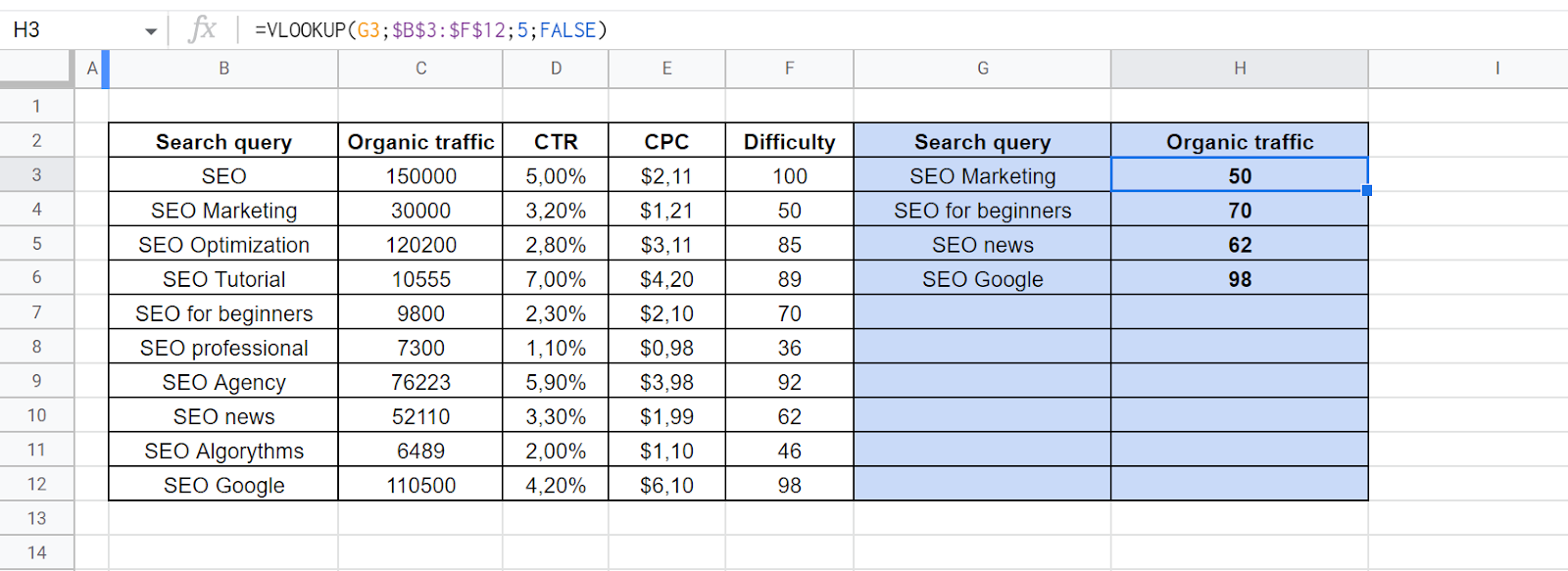
For example, we have selected keywords from a large table and want to add optimization complexity to them. The formula allows you to reduce manual work. It will look like this:
=VLOOKUP(G3;$B$3:$F$12;5;FALSE)
A useful tip: You can fill in cells automatically. Click on a cell containing a formula and hover over the square in the bottom right corner. When the cursor image changes, hold down the left mouse button and drag the formula to all the cells you need.
In this case, all references will be adjusted automatically. This is a convenient option for selecting the desired value. However, the array to be searched must be unchanged. Please note: to keep it in this form, we have marked the column names and row numbers with a dollar sign. To do this, hover over the array address in the formula and press F4 on your keyboard.
QUERY Data Sets Using SQL Queries
How it works: It allows you to create queries in the SQL database programming language. It is used to process data in this document or external sources.
Syntax: =QUERY(range, sql_query), where:
- range — the row in which the check is performed;
- sql_query — the query code.
For example, we have an array of URLs with different content types. We are interested in blog posts labeled as “Blog Posts.”
To select only the necessary URLs, we will use the following formula with an SQL query:
=QUERY(DATA!A:B, “select A where B = “Blog Post”)
ARRAYFORMULA to Apply One Formula to Multiple Cells
How it works: It applies the same formula to all cells below in the column.
Syntax: =ARRAYFORMULA(array_formula), where:
- array_formula — the formula to be applied to the array.
For example, we want to calculate the number of clicks, knowing the volume of organic traffic and CTR. To do it for the entire array, you don’t have to repeat the same formula many times. You can use the following function:
=ARRAYFORMULA(C3:C12*D3:D12)
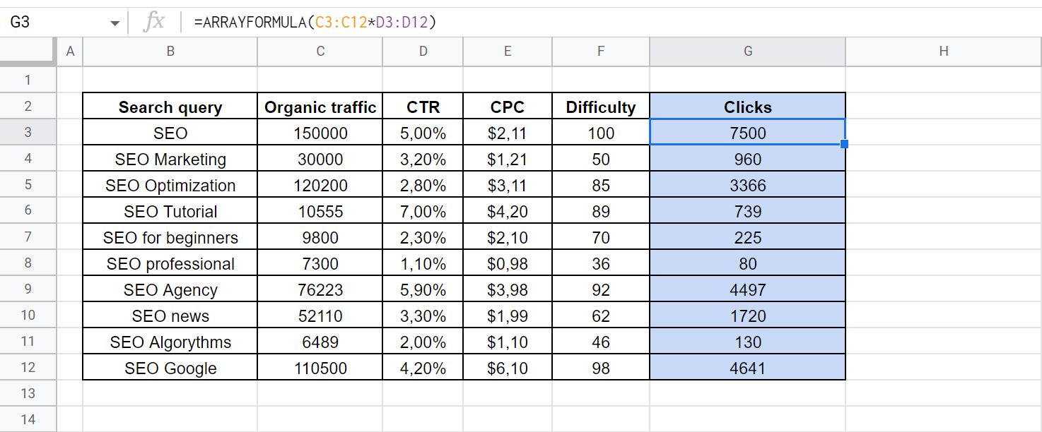
Please note: this time, the formula does not specify cells but rather data rows that are processed by the function.
REGEXTRACT to Extract Data from Strings
How it works: It applies regular expressions to data arrays, just like autocorrect in a text editor or when programming.
Syntax: =REGEXEXTRACT(text, regular_expression), where:
- text — a cell reference;
- regular_expression — the expression to be applied to it.
For example, we have an array of URLs from which we want to extract the address of the base domain. For this purpose, a regular expression with the syntax “^(?:https?:\/\/)?(?:[^@\n][email protected])?(?:www\.)?([^:\/\n]+)” should be used. To avoid errors, use the IFERROR function. The final SEO formula for Google Sheets will look like this:
=IFERROR(ARRAYFORMULA(REGEXEXTRACT(A2:A,”^(?:https?:\/\/)?(?:[^@\n][email protected])?(?:www\.)?([^:\/\n]+)”)),””)
A useful tip: if you’re not familiar with regular expressions, you should check out the RegexR resource for a detailed description of their syntax.
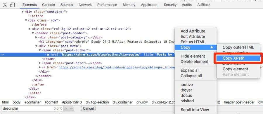
IMPORTXML to Scrape Data from a Website
How it works: The function follows references and uses the XPath query language to get the required info.
Syntax: =IMPORTXML(url, xpath_query), where.
- url — the address of the cell containing the link;
- xpath_query — an XPath query.
For example, we want to use Google Sheets XML formula for SEO ranks by extracting meta tags from them. To get the Title, you will need to use the following query:
=IMPORTXMLA2,“//title”)
A useful tip: We recommend an XPath tutorial to learn syntax. Moreover, you can get the necessary queries in Google Chrome developer mode. To do it, right-click the element you need and select this action:
Google Sheets formulas are a powerful tool for free SEO analytics
With a bit of skill, patience, and practice, you’ll be able to create search engine optimization reports that are as good as expensive paid services. Using Google Sheets formulas for SEO rankings, managing data arrays, and collecting data will save you much time and allow you to focus on important tasks. And that’s not all because spreadsheets support macros. But this is a topic for another article.
FAQ
What Are the Basic SEO Formulas in Google Sheets?
For counting and adding by conditions, COUNTIF and SUMIF are very useful functions. Use IF for checking if a condition is met, SPLIT for splitting cells, and CONCATENATE for merging.
Can You Use Excel Formulas in Google Sheets for SEO?
You can use only those Excel formulas that use basic mathematical operations such as addition, multiplication, etc. More complex functions differ in syntax.
How Do I Create an SEO Formula in Google Sheets?
Select a cell, enter the “=” sign, the desired function, and its parameters. For referring to cells or rows, you should type their addresses in the appropriate part of the formula.


More Like This

Website CMS Checker

Free Backlink Generator